Excelcopy and Paste Without Having to Choose Copy Again

Copying and pasting are probably one of the most used actions in an Excel spreadsheet.

But when it comes to filtered data, copy-pasting data is not always shine.

Ever tried pasting something to a tabular array that has been filtered? It'due south non every bit easy as it sounds.

In this tutorial, I will show yous how to copy information from a filtered dataset and how to paste in a filtered cavalcade while skipping the hidden cells.

• Copying from a Filtered Column Skipping the Hidden Cells
• Pasting a Single Cell Value to All the Visible Rows of a Filtered Cavalcade
• Two Ways to Paste a Set of Values to Visible Rows of a Filtered Column
  • Using a Formula
  • Using VBA Macro Lawmaking

Copying from a Filtered Column Skipping the Subconscious Cells

Suppose you accept the below dataset:

Given the above tabular array, say you want to copy all the rows of employees from the IT department but.

For this, you can apply a filter to your table as follows:

1. Select the entire table.
2. From the Data tab, select the 'Filter' button under the 'Sort & Filter' group.
3. Y'all will notice small-scale arrows on every prison cell of the header row. These are meant to help you filter your cells. Y'all tin click on whatever pointer to choose a filter for the corresponding column.
4. In this instance, we want to filter out only the rows that comprise the Department "Information technology". And so, select the arrow next to the Department header and uncheck the boxes next to all the departments, except "IT". You can but uncheck "Select All" to quickly uncheck everything then just select "IT".
5. Click OK. You will now see only the rows with Department "IT".

Now, copying from a filtered table is quite straightforward. When you copy from a filtered column or table, Excel automatically copies only the visible rows.

So, all you demand to practice is:

1. Select the visible rows that you desire to copy.
2. Press CTRL+C or correct-click->Copy to re-create these selected rows.
3. Select the commencement cell where yous want to paste the copied cells.
4. Printing CTRL+Five or right-click->Paste to paste the cells.

This should crusade just the visible rows from the filtered tabular array to go pasted.

Occasionally you might come across issues in copying the visible rows, peculiarly when working with Subtotals or similar features.

In such cases, copying merely the visible rows is quite easy also. Here'due south what you need to practice:

1. Select the visible rows that you lot want to copy.
2. Press ALT+; (ALT key and semicolon key together). If you're on a Mac, press Cmd+Shift+Z. This shortcut lets you select just the visible rows, while skipping the hidden cells.
3. Printing CTRL+C or right-click->Copy to copy these selected rows.
4. Select the outset prison cell where you want to paste the copied cells.
5. Press CTRL+Five or right-click->Paste to paste the cells.

So you see copying from filtered columns is quite straightforward.

Just you can't say the same when it comes to pasting to a filtered column.

Pasting a Single Cell Value to All the Visible Rows of a Filtered Cavalcade

When it comes to pasting to a filtered column, in that location may exist two cases:

• You might desire to paste a single value to all the visible cells of the filtered column.
• You might want to paste a set of values to visible cells of the filtered column.

For the start case, pasting into a filtered column is quite like shooting fish in a barrel.

Permit'south say nosotros desire to supervene upon all the cells that have Department = "IT" with the total form: "Data Technology".

For this, you can type the give-and-take "Information technology" in any blank cell, copy information technology, and paste it to the visible cells of the filtered "Department" Column. Here's a footstep-by-pace on how to practise this:

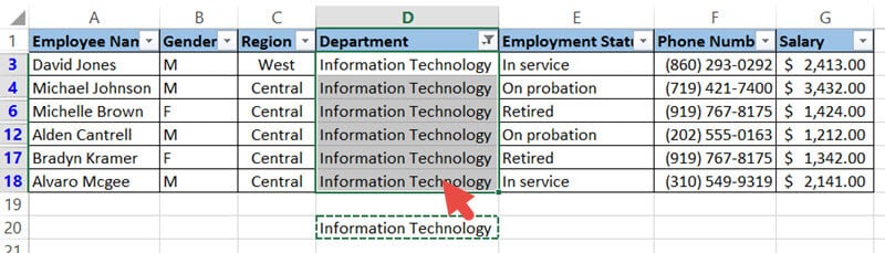
1. Select a blank cell and blazon the words "Information Engineering".
2. Copy it by press CTRL+C or Right click->Copy.
3. Select all the visible cells in the column with the "Department" header.
4. Paste the copied value past pressing CTRL+V or Right click->Paste.

You lot will discover the value "Information Engineering science" pasted to only the visible cells of the column "Department".

To verify this, remove the filter by selecting the Data->Filter. Notice that all the other cells of the "Department" cavalcade remain unchanged.

2 Ways to Paste a Set of Values to Visible Rows of a Filtered Cavalcade

Now let's run into what happens when you want to paste a set of values to the visible cells of a filtered column. Say you want to paste a list of salaries for but the rows containing Department="It".

If you endeavour copying these cells and pasting them to the filtered Salary cavalcade, you will probably get an error bulletin like "The command cannot be used on multiple selections".

This is considering you cannot paste to cells in a range that contains subconscious rows or columns. Information technology's one of Excel'south limitations. There'southward no way around that, but there are some tricks that you tin use to go this washed.

Hither are ii tricks that y'all can employ to paste a prepare of values to a filtered column, skipping the hidden cells.

Pasting a Ready of Values to Visible Rows of a Filtered Column – Using a Formula

In this method, we use a formula to merely copy the value of the jail cell to the destination prison cell.

For the above instance (where you want to copy a ready of salary values to only the rows of with Section= "Information technology"), hither are the steps you need to follow:

1. Press the equal sign ('=') in the first cell of the column you want to paste to (G3).
2. At present select the first jail cell from the listing you lot want to re-create (H3 in our example).
3. This will just create a reference to the cell. Yous should come across the formula: =H3 in cell G3.
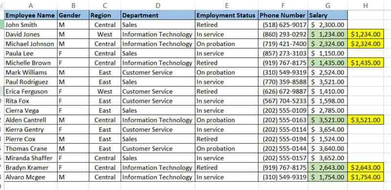
4. Copy this formula down past dragging downwardly the fill handle (at the bottom right corner of jail cell G3). This should paste the formula only to the visible cells of column G.
5. To verify this, remove the filter by selecting Data->Filters. Here'southward an image of column G without filters after the re-create-paste operation. To make it clearer for you lot to meet, I've highlighted the copied cells in lite light-green.
6. Now what you copied were just references to the original cells. So if you try to remove the original cells in one case you're done re-create-pasting, the copied values will disappear from column One thousand too.
7. To avoid this, y'all need to paste these formula results as values. This is quite piece of cake. While you're in the unfiltered mode, re-create all the cells of column One thousand, right-click and select 'Paste Values' from the popup menu.
8. That's it, you tin at present get alee and delete the original values.

Pasting a Gear up of Values to Visible Rows of a Filtered Column – Using VBScript

This is a fairly easier and quicker method. All y'all demand to do is copy the VBScript given beneath into your programmer window and run it.

Sub paste_to_filtered_col() Dim southward As Range Dim visible_source_cells As Range Dim destination_cells Every bit Range Dim source_cell Equally Range Dim dest_cell As Range Set southward = Application.Selection s.SpecialCells(xlCellTypeVisible).Select Set visible_source_cells = Application.Selection Set destination_cells = Application.InputBox("Please select the destination cells:", Blazon:=8) For Each source_cell In visible_source_cells source_cell.Copy For Each dest_cell In destination_cells If dest_cell.EntireRow.RowHeight <> 0 And then dest_cell.PasteSpecial Gear up destination_cells = dest_cell.Offset(1).Resize(destination_cells.Rows.Count) Exit For End If Next dest_cell Next source_cell End Sub

Follow these steps to employ the above code:

1. Select all the rows you need to filter (including the column headers).
2. From the Programmer Menu Ribbon, select Visual Bones.
3. Once your VBA window opens, Click Insert->Module and paste the above lawmaking in the module window.

Your macro is at present fix to run. To run the code:

1. Offset, select the cells that you want to copy.
2. Run the script by navigating to Developer->Macros-> paste_to_filtered_col
3. The code will enquire you to select your destination cells (where you lot desire to paste the copied cells).
4. Select the cells and click OK.

Your selected cells will at present be copied and pasted to the destination cells. You tin can get ahead and delete the original cells if y'all desire.

You can also create a small shortcut (using the Quick Access Toolbar) to run your macro whenever you lot demand it. Here's how:

1. Click the Customize Toolbar arrow, which you'll find higher up Excel's carte du jour ribbon.
2. Select 'More Commands' from the dropdown card that appears.
3. This will open the 'Excel Options' dialog box.
4. Click on the drib-down list beneath 'Choose Commands From' and select 'Macros'.
5. Select the proper noun of the macro you created. In our case, it'southward 'ThisWorkbook.paste_to_filtered_col' Click on the 'Add>>' button.
6. Click OK.

You'll now get a Quick Access macro push button to quickly run your macro with a single click.

Whenever you need to copy and paste a set of cells to a filtered column, just select your source cells, click on this created button and then select the destination cells.

When you click OK, you lot should get your source cells copied into your selected destination cells.

So this is how yous can copy and paste in a filtered column while skipping the hidden rows.

I hope you establish this tutorial useful!

Other Excel tutorials you may similar:

• How to Delete Filtered Rows in Excel (with and without VBA)
• How to Filter as Yous Blazon in Excel (With and Without VBA)
• How to Unsort in Excel (Revert Back to Original Data)
• How to Hide Rows based on Jail cell Value in Excel
• How to Compare 2 Cells in Excel?

allenteve1963.blogspot.com

Source: https://spreadsheetplanet.com/paste-filtered-column-skipping-hidden-cells/

Share this post